The Hubbard Model

The minimal model of reference for the cuprates — one hopping amplitude and one on-site repulsion — together with its particle–hole symmetry, Green's functions, and the two limits (atomic and non-interacting) that already reveal the Mott insulator.

Methods Green's functionsTight binding

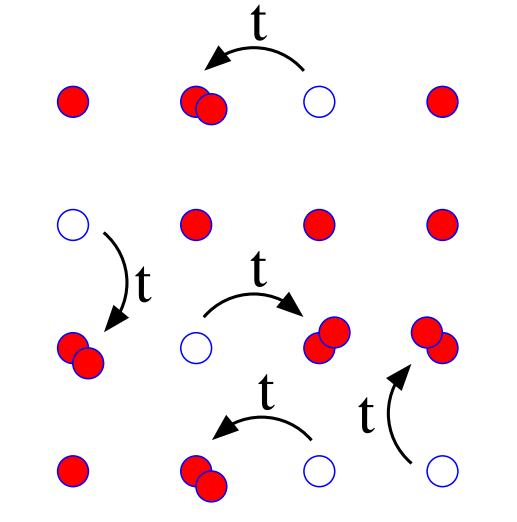
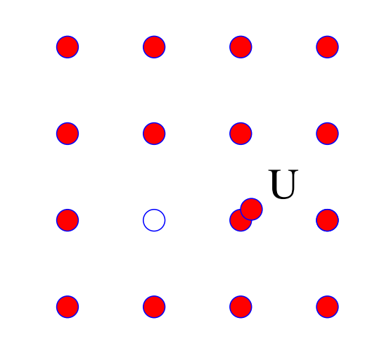
The Hubbard model is the standard theoretical framework for correlated electrons in cuprates. It is a tight-binding model in which electrons are largely localized on atomic sites and move only by tunnelling, with hopping amplitude . Electron–electron interactions enter as an on-site Coulomb repulsion , on a square lattice of copper atoms with a single active orbital per site — the single-band Hubbard model. Working in the grand canonical ensemble on sites, with ,

where the last term is the chemical potential .

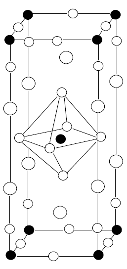
The justification: in-plane Cu–Cu distances are much shorter than the spacing to the oxygen atoms in the insulating layers, so the essential physics happens within the planes; the spacer layers act as charge reservoirs. Each copper hosts a shell whose near-degeneracy is split by the crystal field, leaving a single active orbital. Hopping is actually mediated by the bridging oxygens, but is conventionally written as direct Cu–Cu hopping.

Particle–hole symmetry

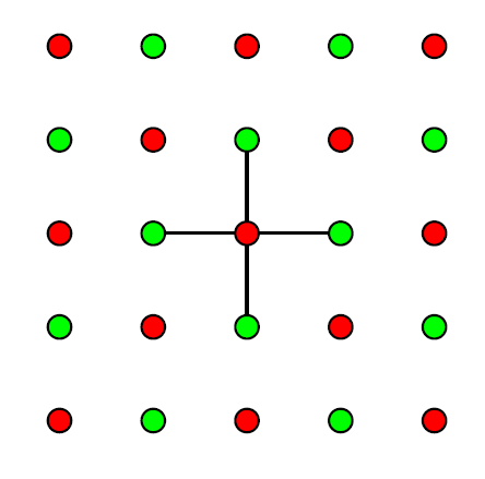
Bipartite lattices — such as the square and cubic lattices — split into two sublattices and so that every site of one neighbours only sites of the other. This structure naturally supports antiferromagnetic order: spin-up and spin-down electrons can occupy separate sublattices without violating the Pauli principle.

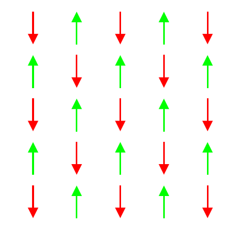
Introduce the particle–hole transformation (PHT):

The arrow means “replace the left operator by the right one in ”. The factor depending on the sublattice of site ; for nearest neighbours on opposite sublattices, . The operator identities follow:

The terms of the Hamiltonian therefore transform as

describes the dynamics of holes; is invariant under PHT only if . Consider now the equivalent symmetric form of the Hamiltonian,

which differs from the standard form only by a shift of and a constant, since

In this form both kinetic and interaction terms are PHT-invariant; only the chemical-potential term changes sign (up to a constant),

so the Hamiltonian is PHT-invariant only at . Defining the average site occupancy

PHT sends , i.e. . Because the system is particle–hole symmetric at , , hence

That is, corresponds to half-filling.

Green’s functions

Green’s functions are the correlation functions at the centre of many-body theory. Labelling the eigenstates of the full by , the Green’s function (GF) is

where is the time-ordering operator (not temperature), e.g. for a generic operator ,

and the expectation value is taken in the ground state () or the canonical ensemble (finite ). Operators evolve in the Heisenberg picture,

The closely related spectral function, central to experimental observables, is

where is the Fourier transform of the retarded Green’s function

Here is the anticommutator (fermions) or commutator (bosons), and is the Heaviside step. is a resolved density of states — the probability of finding a particle in state with excitation energy . Below we compute and two ways: via the imaginary-time (Matsubara) formalism, and via the spectral (Lehmann) representation.

The single-site (atomic) limit

To gain insight into the deceptively simple but analytically hard Hubbard model, take — no hopping — giving the single-site Hubbard model,

Here the number operators commute with and with each other, , so is separable and each site is analysed independently:

This is the atomic limit of the Anderson impurity model (AIM), describing an isolated ion:

where and create conduction and localized electrons, is the hybridization, the conduction dispersion, the impurity level, and the on-site repulsion. The AIM atomic limit is

Rewriting

the last term is a constant shift, and the two Hamiltonians coincide under . We proceed with . With a single site, the configurations are

(first/second entry = number of spin-up/down electrons), with energies , , , . The energy to add or remove an electron from the two-fold degenerate level is

Provided , i.e. , the singly occupied states lie lowest: the ground state is a localized single electron carrying a magnetic moment, with charge transport suppressed — already the hallmark of a Mott insulator.

The Mott insulator: an insight

Thermodynamics starts from the partition function

The four atomic-state energies, in Hubbard parameters, are

At these simplify to a particle–hole symmetric spectrum,

and the partition function becomes

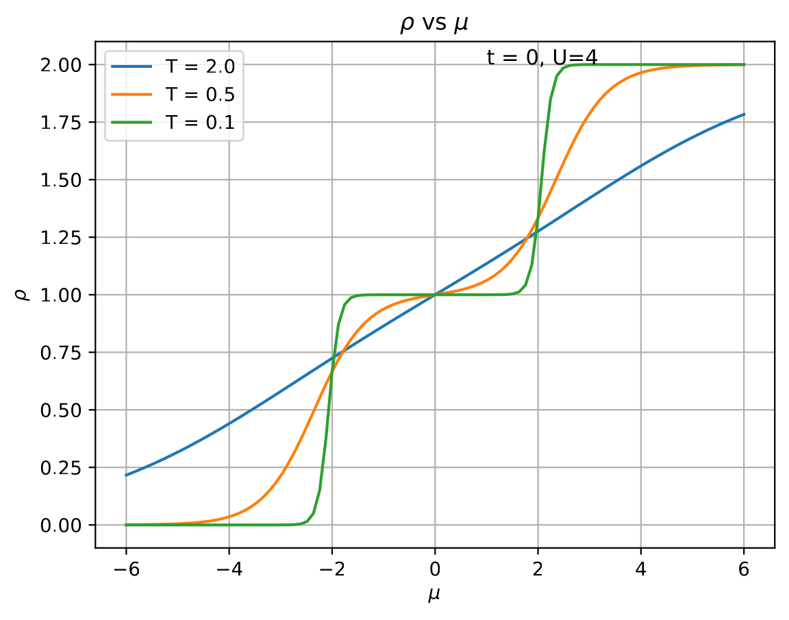
The average occupation follows,

At the system is half-filled, . Plotting for at various temperatures shows, at low , a plateau pinned at around : the Mott gap. Adding or removing an electron costs energy of order ; raising blurs the gap.

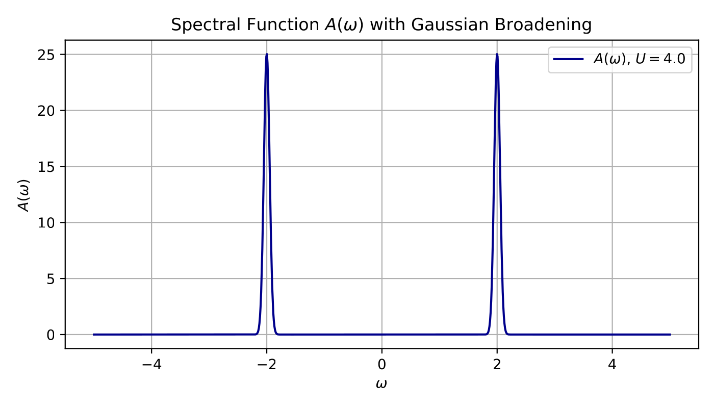
The spectral function (single site)

It is convenient to work on the imaginary axis and analytically continue to the real axis afterwards.

Imaginary-time approach. The Matsubara Green’s function is

with the imaginary-time ordering operator and . At ,

Fourier transforming with ,

For fermions only odd Matsubara frequencies appear; using ,

Analytic continuation gives the retarded function

and Cauchy’s identity

yields the spectral function

Lehmann representation. The same result follows from the Lehmann form, which expresses through the eigenstates of the full interacting ,

At , only and contribute, giving

matching the earlier and the same . The two Dirac ‘s are the minimal excitation energies to add or remove an electron from the singly-occupied ground state, : charge transport requires overcoming a finite barrier, so the system is insulating.

Finally, the single-site spin-up occupation,

which as ; by particle–hole symmetry , so , the lowest-energy half-filled configuration.

The non-interacting limit ()

In the opposite limit the Hamiltonian reduces to tight-binding,

Lattice-translation invariance lets us diagonalize in momentum space,

Using ,

i.e. in compact form

with lattice constant . The dispersion gives a density of states

(with normalized by the Brillouin-zone volume) that diverges logarithmically at — a van Hove singularity. At half-filling, electrons fill of the spin-resolved states, so band theory predicts a conductor.

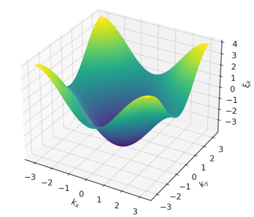
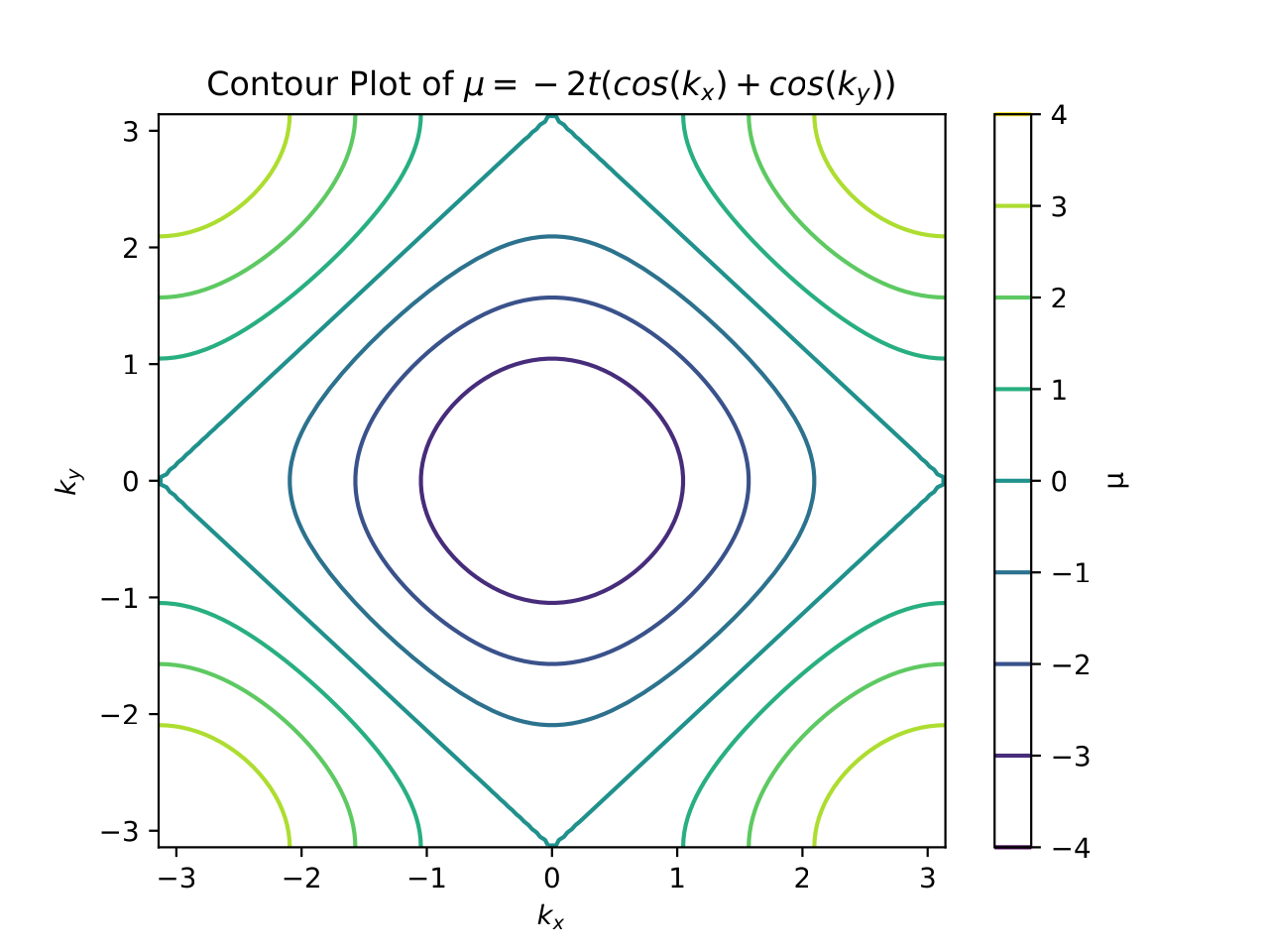
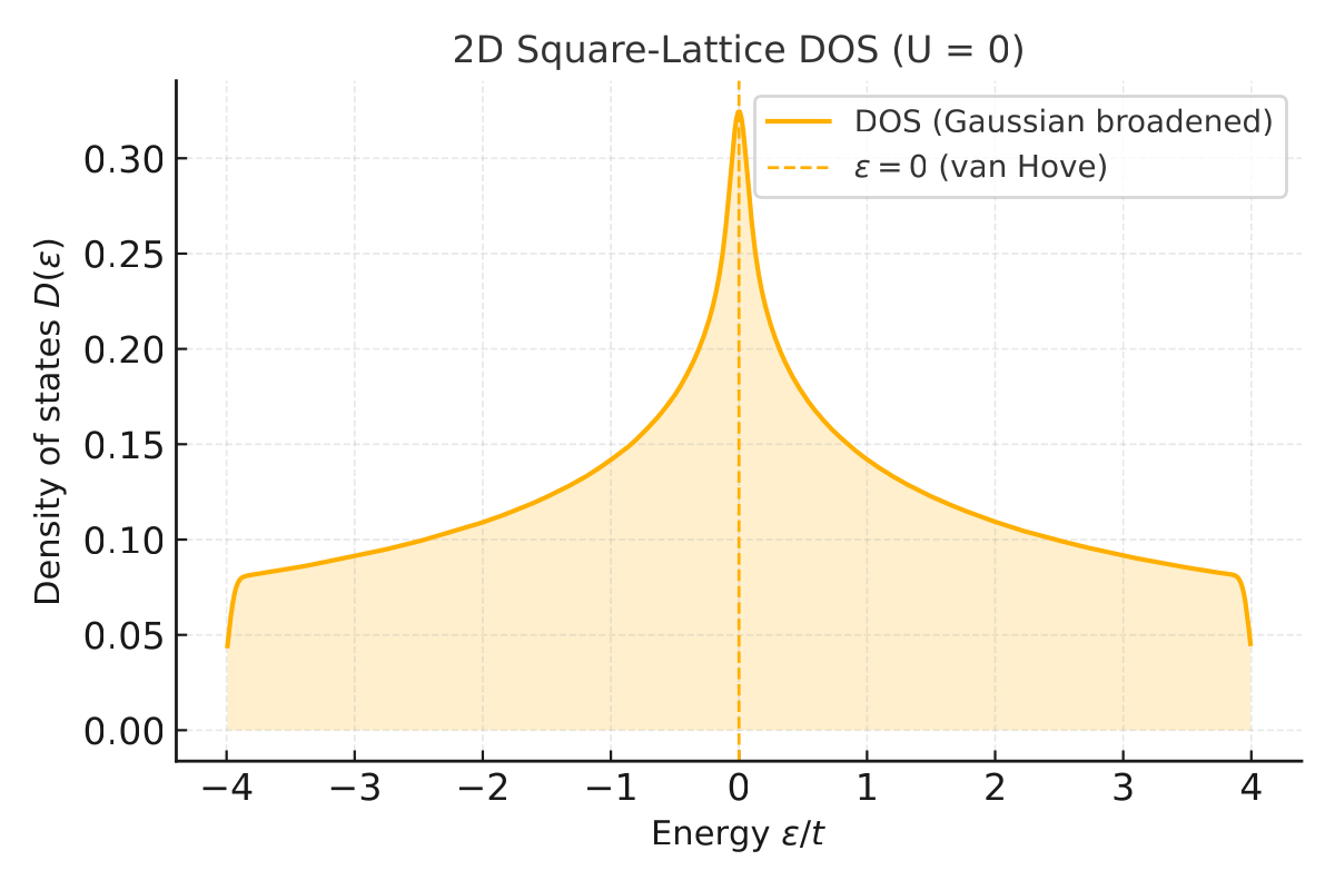
The Fermi surface exhibits, at , perfect nesting at : large segments map onto each other under translation by . This enhances the susceptibility to antiferromagnetic ordering at and motivates the mean-field treatment of the magnetization in the weak-coupling topic.

The spectral function ()

The retarded Green’s function is

with spectral function

sharply peaked at the quasiparticle energy — the spectral weight of a non-interacting particle is a single coherent -peak. Restoring is the whole story of this subject: it is what turns this sharp band metal into a Mott insulator, the subject of the weak- and strong-coupling topics, and the DMFT study that follows.